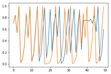
Illustration of the logistic map,
At , a stable period orbit is born. At a stable period orbit is born. As continues to increase, the period doublings continue until after which chaotic dynamics begin to occur, interspersed with periodic windows.
The Feigeinbaum constant is the ratio of subsequent differences between the values of at which the period doubles, as approaches infinity.
import numpy as np
import matplotlib.pyplot as plt
import pylab

def f(x, R):
    return R * x * (1 - x)

def run_simulation(R, x_0, num_steps):
    x_list = np.zeros(num_steps)
    x_list[0] = x_0
    for t in range(num_steps-1):
        x_list[t+1] = f(x_list[t], R)
    return x_list

def plot_two(x_list, y_list):
    plt.plot(x_list)
    plt.plot(y_list)
x_list = run_simulation(R=4, x_0=0.7, num_steps=50)
y_list = run_simulation(R=4, x_0=0.70001, num_steps=50)plot_two(x_list, y_list)